Estimating Hydropower with the Reservoir Module

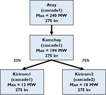
This notebook shows an example of estimating daily hydropower time series given a water system. Here, we will work with a system called “complex_river”, comprising four reservoirs: Atay, Kamchay, Kirirom1, and Kirirom2. These reservoirs are situated in a cascade. Water flow from Kamchay are diverted 25% to Kirirom1 and 75% to Kirirom2. Hydropower capacities are shown in the figure below.

The following code imports necessary libraries and displays a diagram of the ‘complex_river’ water system, illustrating reservoir connections and hydropower capacities. Data files for this case study, called “complex_river”, can be found here. Please download them to a folder on your local machine.

import os
from IPython.display import Image, display
from pownet.folder_utils import get_pownet_dir

project_root = get_pownet_dir()
image_path = os.path.join(project_root, "images", "complex_river.png")
display(Image(filename=image_path))

Setup: Input/Output Folders

First, we specify the directory containing the input data using input_folder. If simulation results need to be saved, we also define the output_folder. PowNet requires the following CSV files:

• reservoir_unit.csv contains information on the characteristics of reservoirs

• inflow.csv contains the daily inflow to each reservoirs

• minimum_flow.csv contains the daily minimum flow from each reservoirs

• flow_paths.csv contains the system topology – the water flow paths

This code block imports the ReservoirManager and defines essential paths. It sets up the input_folder where PowNet will look for model data (e.g., CSV files for the ‘complex_river’ model) and an output_folder for saving simulation results. Note: If PowNet was installed via pip, or if your data resides in a different location, you may need to adjust the input_folder path accordingly.

import os
from pownet.reservoir import ReservoirManager

input_folder = os.path.join(project_root, "model_library")
output_folder = os.path.join(project_root, "outputs")

# Define the specific model name
model_name = "complex_river"
input_folder = os.path.join(input_folder, model_name)

Reservoir simulation

The operation of downstream reservoirs is influenced by the operations of those upstream. The ReservoirManager class orchestrates the simulation sequence, commencing with the most upstream reservoirs and progressing downstream. The subsequent code block demonstrates loading reservoir parameters from the previously defined CSV files and executing a simulation to generate time-series data of reservoir dynamics (e.g., water levels, flow, hydropower generation).

Here, we initialize the ReservoirManager, load the reservoir characteristics and system topology from CSV files located in the input_folder, and then run the reservoir simulation based on the loaded data and predefined operational rules.

reservoir_manager = ReservoirManager()
reservoir_manager.load_reservoirs_from_csv(input_folder)
reservoir_manager.simulate()

After the simulation, we retrieve the simulated daily hydropower generation time series for all reservoirs as a pandas DataFrame. We then display the first 5 days of this data, rounded to the nearest whole number, for a quick review.

hydropower_df = reservoir_manager.get_hydropower_ts()
hydropower_df.round(0).head()

	atay	kamchay	kirirom1	kirirom2
1	752.0	569.0	288.0	432.0
2	1804.0	1423.0	288.0	432.0
3	1796.0	1406.0	288.0	432.0
4	1788.0	1396.0	288.0	432.0
5	1779.0	1384.0	288.0	432.0

Finally, to visualize the results for a specific reservoir, we access the ‘atay’ reservoir object from the ReservoirManager and then generate and display a plot summarizing its state variables (e.g., water level, inflow, outflow, generation) over the simulation period. Of course, we can do this for the other three reservoirs as well.

atay_reservoir = reservoir_manager.reservoirs["atay"]
atay_reservoir.plot_state() # Include the output_folder argument if you want to save the plot